After performing a study, you can correctly conclude there is an effect or not, but you can also incorrectly conclude there is an effect (a false positive, alpha, or Type 1 error) or incorrectly conclude there is no effect (a false negative, beta, or Type 2 error).
The goal of collecting data is to provide evidence for or against a hypothesis.
Take a moment to think about what ‘evidence’ is – most researchers I ask can’t
come up with a good answer. For example, researchers sometimes think p-values are evidence, but p-values are only correlated with
evidence.
Evidence in science is necessarily relative. When data is more likely assuming one model is true
(e.g., a null model) compared to another model (e.g., the alternative model),
we can say the model provides evidence for the null compared to the alternative
hypothesis. P-values only give you the
probability of the data under one model – what you need for evidence is the relative
likelihood of two models.
Bayesian and likelihood approaches should be used when you
want to talk about evidence, and here I’ll use a very simplistic likelihood
model where we compare the relative likelihood of a significant result when the
null hypothesis is true (i.e., making a Type 1 error) with the relative
likelihood of a significant result when the alternative hypothesis is true
(i.e., *not* making a Type 2 error).
Let’s assume we have a ‘methodological fetishist’ (Ellemers, 2013) who is adamant about controlling their alpha
level at 5%, and who observes a significant result. Let’s further assume this
person performed a study with 80% power, and that the null hypothesis and
alternative hypothesis are equally (50%) likely. The outcome of the study has a
2.5% probability of being a false positive (a 50% probability that the null
hypothesis is true, multiplied by a 5% probability of a Type 1 error), and a
40% probability of being a true positive (a 50% probability that the
alternative hypothesis is true, multiplied by an 80% probability of finding a
significant effect).
The relative evidence for H1 versus H0 is 0.40/0.025 = 16. In
other words, based on the observed data, and a model for the null and a model
for the alternative hypothesis, it is 16 times more likely that the alternative
hypothesis is true than that the null hypothesis is true. For educational
purposes, this is fine – for statistical analyses, you would use formal
likelihood or Bayesian analyses.
Now let’s assume you agree that providing evidence is a very
important reason for collecting data in an empirical science (another goal of data
collection is estimation – but I’ll focus on hypothesis testing here). We can now ask
ourselves what the effect of changing the Type 1 error or the Type 2 error
(1-power) is on the strength of our evidence. And let’s agree that we will
conclude that whichever error impacts the strength of our evidence the most, is
the most important error to control. Deal?
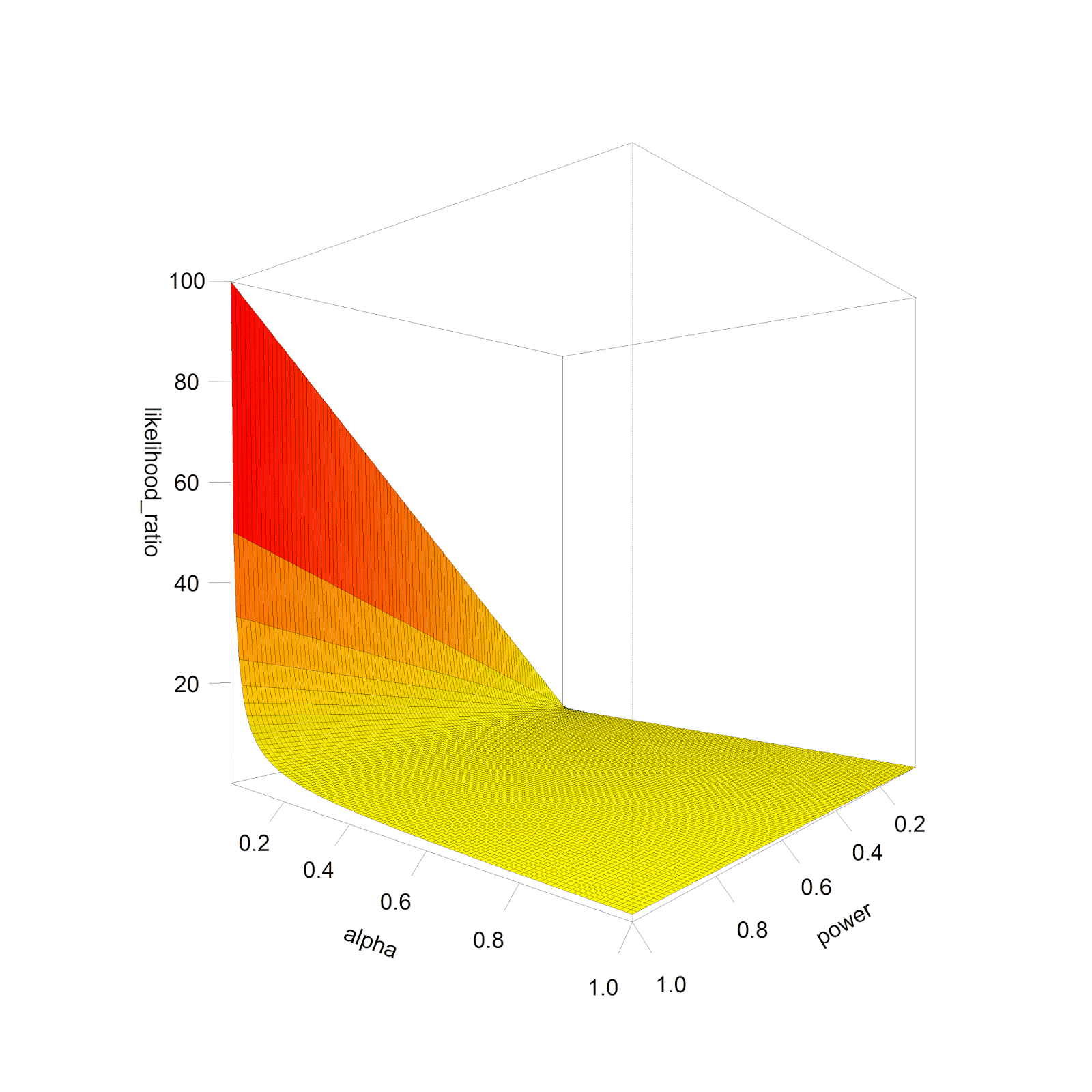
We can plot the relative likelihood (the probability a
significant result is a true positive, compared to a false positive) assuming
H0 and H1 are equally likely, for all levels of power, and for all alpha
levels. If we do this, we get the plot below:
Or for a rotating version (yeah, I know, I am an R nerd):

So when is the evidence in our data the strongest? Not
surprisingly, this happens when both types of errors are low: the alpha level
is low, and the power is high (or the Type 2 error rate is low). That is why
statisticians recommend low alpha levels and high power. Note that the shape of
the plot remains the same regardless of the relative likelihood H1 or H0 is
true, but when H1 and H0 are not equally likely (e.g., H0 is 90% likely to be
true, and H1 is 10% likely to be true) the scale on the likelihood ratio axis
increases or decreases.
Now for the main point in this blog post: we can see that an
increase in the Type 2 error rate (or a reduction in power) reduces the
evidence in our data, but it does so relatively slowly. However, we can also
see that an increase in the Type 1 error rate (e.g., as a consequence of
multiple comparisons without controlling for the Type 1 error rate) quickly
reduces the evidence in our data. Royall (1997)
recommends that likelihood ratios of 8 or higher provide moderate evidence, and
likelihood ratios of 32 or higher provide strong evidence. Below 8, the
evidence is weak and not very convincing.
If we calculate the likelihood ratio for alpha = 0.05, and
power from 1 to 0.1 in steps of 0.1, we get the following likelihood ratios: 20,
18, 16, 14, 12, 10, 8, 6, 4, 2. With 80% power, we get the likelihood ratio of
16 we calculated above, but even 40% power leaves us with a likelihood ratio of
8, or moderate evidence (see the figure above). If we calculate the likelihood ratio for power = 0.8
and alpha levels from 0.05 to 0.5 in steps of 0.05, we get the following
likelihood ratios: 16, 8, 5.3, 4, 3.2, 2.67, 2.29, ,2, 1.78, 1.6. An alpha
level of 0.1 still yields moderate evidence (assuming power is high enough!)
but further inflation makes the evidence in the study very weak.
To conclude: Type 1 error rate inflation quickly destroys
the evidence in your data, whereas Type 2 error inflation does so less severely.
Type 1 error control is important if we care
about evidence. Although I agree with Fiedler, Kutzner,
and Kreuger (2012) that a Type 2 error is also
very important to prevent, you simply can not ignore Type 1 error control if
you care about evidence. Type 1 error control is more important than Type 2
error control, because inflating Type 1 errors will very quickly leave you with
evidence that is too weak to be convincing support for your hypothesis, while
inflating Type 2 errors will do so more slowly. By all means, control Type 2 errors - but not at the expense of Type 1 errors.
I want to end by pointing out that Type 1 and Type 2 error
control is not a matter of ‘either-or’. Mediocre statistics textbooks like to
point out that controlling the alpha level (or Type 1 error rate) comes at the expense of the beta (Type
2) error, and vice-versa, sometimes using the horrible seesaw metaphor below:

Image from: http://www.statisticsfromatoz.com/blog/statistics-tip-of-the-week-the-alpha-and-beta-error-seesaw
But this is only true if the sample size is fixed. If you
want to reduce both errors, you simply need to increase your sample size, and
you can make Type 1 errors and Type 2 errors are small as you want, and contribute
extremely strong evidence when you collect data.
Ellemers, N. (2013). Connecting the dots: Mobilizing theory to reveal
the big picture in social psychology (and why we should do this): The big
picture in social psychology. European Journal of Social Psychology, 43(1),
1–8. https://doi.org/10.1002/ejsp.1932
Fiedler, K., Kutzner, F., & Krueger,
J. I. (2012). The Long Way From -Error Control to Validity Proper: Problems
With a Short-Sighted False-Positive Debate. Perspectives on Psychological
Science, 7(6), 661–669. https://doi.org/10.1177/1745691612462587
Royall, R. (1997). Statistical
Evidence: A Likelihood Paradigm. London ; New York: Chapman and Hall/CRC.